Toy Example

Assorted overview of some more niche functionality.

Prelude

from importlib import reload as re

import landau as ld
import landau.interpolate as ldi
import landau.calculate as ldc

import numpy as np

import matplotlib.pyplot as plt

import pandas as pd

import seaborn as sns

Toy Example

l1 = ld.TemperatureDependentLinePhase(
    "l0", fixed_concentration=0, temperatures=[1, 750, 1000], free_energies=[2, 1.80, 1.00], interpolator=ldi.PolyFit(3)
)
l2 = ld.TemperatureDependentLinePhase(
    "l1", fixed_concentration=1, temperatures=[1, 750, 1000], free_energies=[3, 2.80, 2.00], interpolator=ldi.PolyFit(3)
)
l3 = ld.TemperatureDependentLinePhase(
    "l2",
    fixed_concentration=0.5,
    temperatures=[1, 750, 1000],
    free_energies=[2.45, 2.00, 1.42],
    interpolator=ldi.PolyFit(3),
)
liq = ld.IdealSolution("liquid", l1, l2)
rliq = ld.RegularSolution("liquid", [l1, l3, l2])

s1 = ld.TemperatureDependentLinePhase(
    "s0", fixed_concentration=0, temperatures=[1, 750, 1000], free_energies=[1.9, 1.6, 1.2], interpolator=ldi.SGTE(2)
)
s2 = ld.TemperatureDependentLinePhase(
    "s1", fixed_concentration=1, temperatures=[1, 750, 1000], free_energies=[2.9, 2.6, 2.2], interpolator=ldi.SGTE(2)
)
s3 = ld.TemperatureDependentLinePhase(
    "s3",
    fixed_concentration=0.4,
    temperatures=[1, 750, 1000],
    free_energies=np.array([2.4, 1.85, 1.45]) - 0.05,
    interpolator=ldi.SGTE(3),
)
sol = ld.IdealSolution("solid", s1, s2)

Ts = np.linspace(50, 1000, 100)

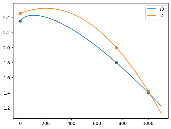
s3.check_interpolation()
l3.check_interpolation()
plt.legend()

/home/ponder/science/phd/dev/landau/landau/interpolate.py:110: OptimizeWarning: Covariance of the parameters could not be estimated
  parameters, *_ = so.curve_fit(G_calphad, x, y, p0=[0] * self.nparam)

<matplotlib.legend.Legend at 0x7fabfc749250>

c = np.linspace(0, 1, 75)[1:-1]
mu = 1 + ld.phases.kB * 4000 * np.log(c / (1 - c))

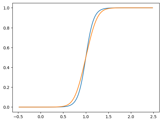
plt.plot(mu, liq.concentration(1000, mu))
plt.plot(mu, rliq.concentration(1000, mu))

[<matplotlib.lines.Line2D at 0x7fab5c928dd0>]

rliq.check_interpolation(750)

# df = ppdt.calc_phase_diagram([liq, s1, s2], np.linspace(50, 1000), mu, refine=True)

from importlib import reload as re

re(ld.phases)
re(ld)

<module 'landau' from '/home/ponder/science/phd/dev/landau/landau/__init__.py'>

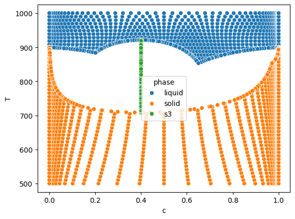
df = ldc.calc_phase_diagram([rliq, sol, s3], np.linspace(500, 1000, 50), mu, refine=True)

sns.scatterplot(data=df.query("stable"), x="c", y="T", hue="phase")

<Axes: xlabel='c', ylabel='T'>

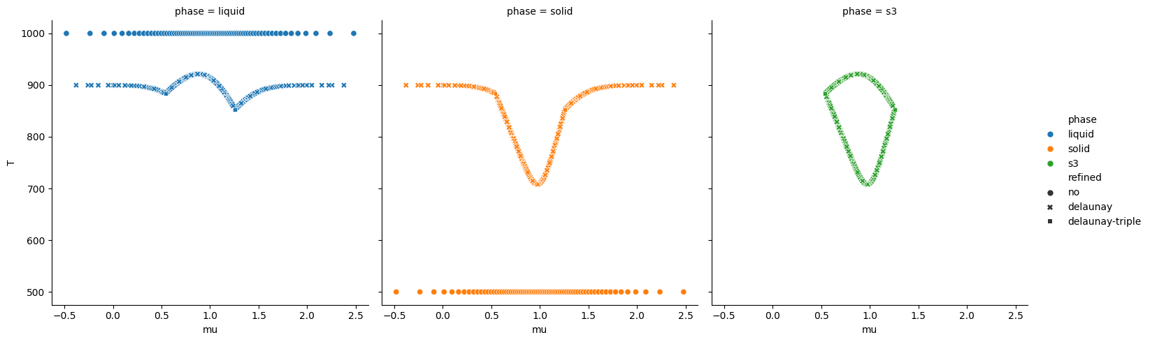
sns.relplot(
    data=df.query("border"),
    x="mu",
    y="T",
    hue="phase",
    col="phase",
    style="refined",
)

<seaborn.axisgrid.FacetGrid at 0x7fab5c9bed50>

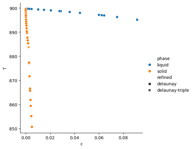
sns.relplot(
    data=df.query("border and 850<T<920 and c<.1"),
    x="c",
    y="T",
    hue="phase",
    # col='phase',
    style="refined",
)

<seaborn.axisgrid.FacetGrid at 0x7fab5c637c50>

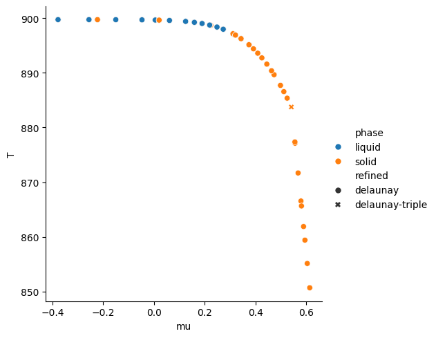
sns.relplot(
    data=df.query("border and 850<T<920 and c<.1"),
    x="mu",
    y="T",
    hue="phase",
    # col='phase',
    style="refined",
)

<seaborn.axisgrid.FacetGrid at 0x7fab5c695cd0>

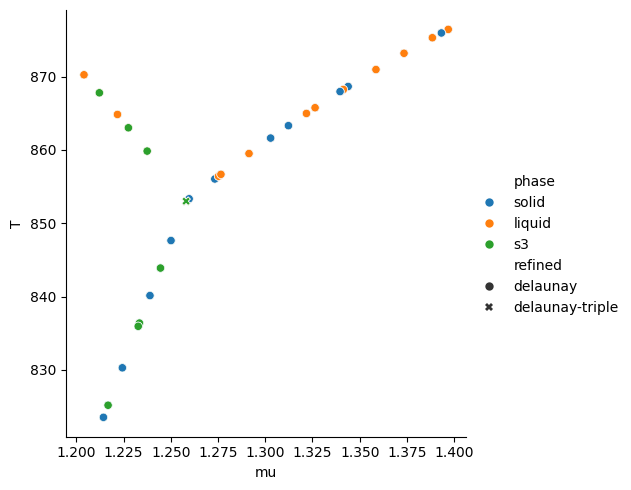
sns.relplot(
    data=df.query("border and 820<T<880 and 1.2<mu<1.4"),
    x="mu",
    y="T",
    hue="phase",
    # col='phase',
    style="refined",
)

<seaborn.axisgrid.FacetGrid at 0x7fab5c6e6d50>

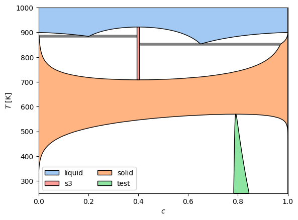
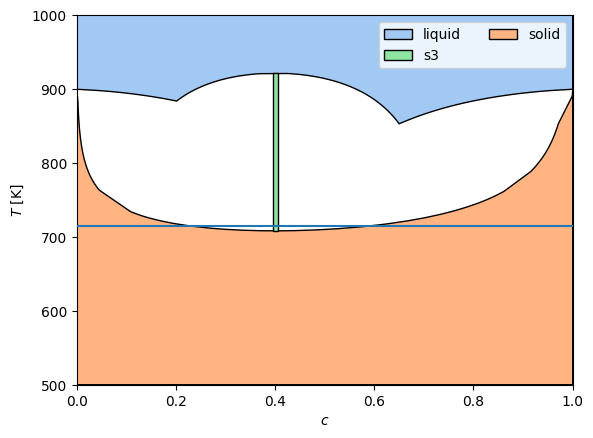
ld.plot_phase_diagram(df)
plt.axhline(714.285714, zorder=10)
# plt.ylim(750, 1000)

<matplotlib.lines.Line2D at 0x7fab5c6ff7d0>

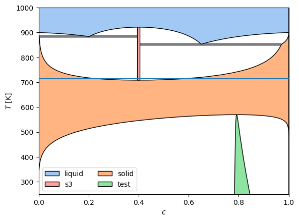
ld.plot_phase_diagram(df, poly_method='tsp', tielines=True)
plt.axhline(714.285714, zorder=10)
# plt.ylim(750, 1000)

<matplotlib.lines.Line2D at 0x7fabe2a0acd0>

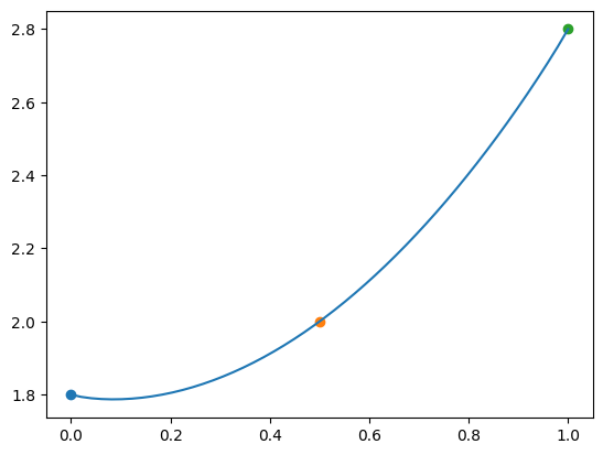
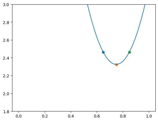
p = ld.InterpolatingPhase(
    "test",
    [
        ld.LinePhase("s0", 0.65, 2.50, 0.00005),
        ld.LinePhase("s0", 0.75, 2.40, 0.00010),
        ld.LinePhase("s0", 0.85, 2.50, 0.00005),
    ],
    num_coeffs=3,
    num_samples=250,
)

p.check_interpolation(750)
plt.ylim(1.8, 3)

(1.8, 3.0)

c = np.linspace(0, 1, 50)[1:-1]
mu = 1 + ld.phases.kB * 4000 * np.log(c / (1 - c))

%%time
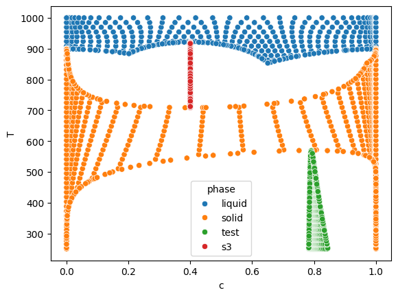
df = ldc.calc_phase_diagram([rliq, sol, p, s3], np.linspace(250, 1000, 50), mu, refine=True)

CPU times: user 24.3 s, sys: 72.6 ms, total: 24.3 s
Wall time: 24.6 s

sns.scatterplot(data=df.query("stable"), x="c", y="T", hue="phase")

<Axes: xlabel='c', ylabel='T'>

%%time
ld.plot_phase_diagram(df, poly_method='tsp', tielines=True)

CPU times: user 4.43 s, sys: 191 ms, total: 4.62 s
Wall time: 4.63 s