Line Phases

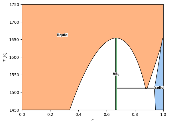
This example adds an intermetallic (or line phase) without solubility to the same setup of the ideal solution example.

Prelude

from landau.phases import LinePhase, IdealSolution
from landau.calculate import calc_phase_diagram
from landau.plot import plot_phase_diagram, plot_1d_T_phase_diagram, plot_1d_mu_phase_diagram, plot_mu_phase_diagram, plot_excess_free_energy

import numpy as np
from scipy.constants import Boltzmann, eV
kB = Boltzmann/eV

import seaborn as sns
import matplotlib.pyplot as plt

Phases Setup

Same phase setup as in IdealSolution.ipynb. Energies and entropies are picked manually to make simple examples.

solid_a = LinePhase('A', fixed_concentration=0, line_energy=-2.0, line_entropy=1.0*kB)
solid_b = LinePhase('B', fixed_concentration=1, line_energy=-3.0, line_entropy=1.5*kB)

solid = IdealSolution('solid', solid_a, solid_b)

liquid_a = LinePhase('A(l)', fixed_concentration=0, line_energy=-1.9, line_entropy=2.5*kB)
liquid_b = LinePhase('B(l)', fixed_concentration=1, line_energy=-2.9, line_entropy=2.2*kB)

liquid = IdealSolution('liquid', liquid_a, liquid_b)

inter = LinePhase('AB$_2$', fixed_concentration=2/3, line_energy=-2.8, line_entropy=1.3*kB)

df = calc_phase_diagram([solid, liquid, inter], Ts=np.linspace(1, 2000, 100), mu=200, keep_unstable=True)

import landau.poly as lp

%%time
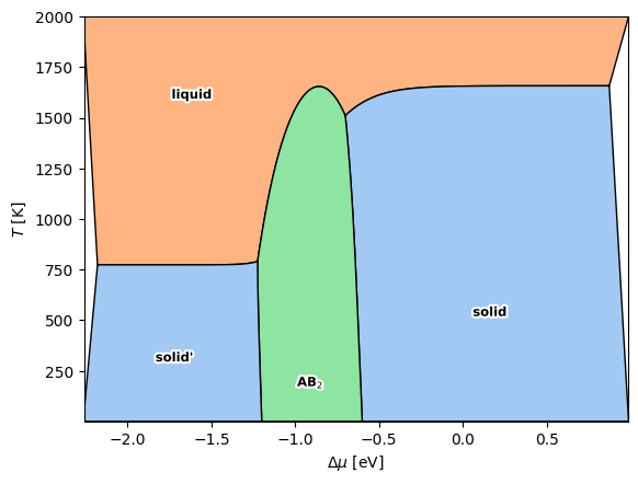
plot_mu_phase_diagram(df, poly_method=lp.FastTsp(duration_seconds=1))

CPU times: user 4.39 s, sys: 475 ms, total: 4.87 s
Wall time: 4.54 s

%%time
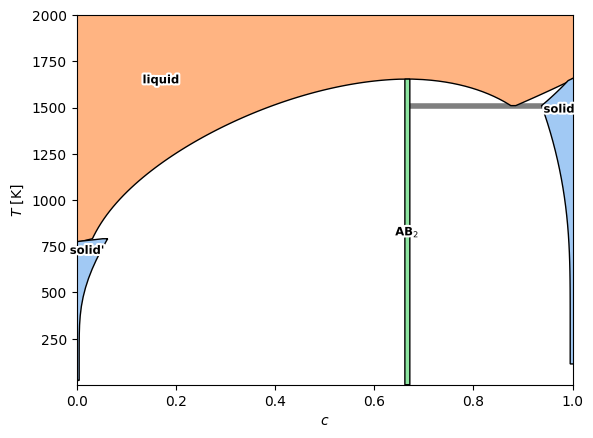
plot_phase_diagram(df, tielines=True)

/home/runner/work/landau/landau/landau/poly.py:69: UserWarning: SegmentFastTsp._make produced an invalid polygon (Self-intersection[0.681215015742246 -2.05233178430845]); repairing it.
  warn(f"{type(self).__name__}._make produced an invalid polygon "
/home/runner/work/landau/landau/landau/poly.py:69: UserWarning: SegmentFastTsp._make produced an invalid polygon (Ring Self-intersection[-0.521516394612764 -1.87569296489371]); repairing it.
  warn(f"{type(self).__name__}._make produced an invalid polygon "

CPU times: user 1.35 s, sys: 12.1 ms, total: 1.36 s
Wall time: 1.35 s

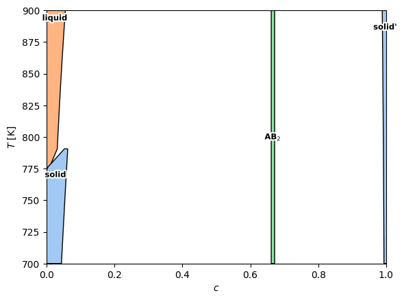
Zoom on Invariant Reactions

df = calc_phase_diagram([solid, liquid, inter], Ts=np.linspace(700, 900, 100), mu=200, keep_unstable=True)

%%time
plot_phase_diagram(df, tielines=True)

CPU times: user 1.16 s, sys: 1.02 ms, total: 1.16 s
Wall time: 1.16 s

df = calc_phase_diagram([solid, liquid, inter], Ts=np.linspace(1450, 1750, 100), mu=200, keep_unstable=True)

%%time
plot_phase_diagram(df, tielines=True)

CPU times: user 1.44 s, sys: 1 ms, total: 1.45 s
Wall time: 1.44 s

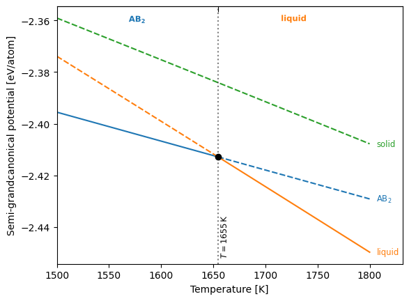
Congruent Melting of Intermetallic Phase

In general, the phase boundaries in a phase diagram demark where the semi-grand potentials are equal across phases. For intermetallics with neglible solubility, we can follow the isopotential lines along temperature to find the exact melting point. landau does this implicitly when calculating the full phase diagram, but we can follow along temperature only, if we print the equilibrium chemical potential from the full calculation above and then recalculate the equilibria at that potential.

ab = df.query('border and phase == "AB$_2$"')
ab.loc[ab['T'].idxmax(),['mu', 'T']]

mu      -0.857277
T     1654.559173
Name: 60568, dtype: float64

df = calc_phase_diagram([solid, liquid, inter], Ts=np.linspace(1500, 1800, 100), mu=-0.858751, keep_unstable=True)

plot_1d_T_phase_diagram(df)

<Axes: xlabel='Temperature [K]', ylabel='Semi-grandcanonical potential [eV/atom]'>

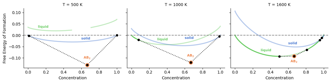
Double Tangent Construction and Free Energies of Formation

landau works entirely in chemical potential space, but the equivalent double tangent constructions can be reconstructed from the dataframes returned from calc_phase_diagram. The example below first calculates three isothermal sections of the phase diagram

import pandas as pd

df = pd.concat([
    calc_phase_diagram([solid, liquid, inter], Ts=T, mu=100, keep_unstable=True)
        for T in [500, 1000, 1600]
], ignore_index=True)

plot_excess_free_energy(df, convex_hull=True)

<seaborn.axisgrid.FacetGrid at 0x7fc9f69137a0>