Ideal Solution

Prelude

from landau.phases import LinePhase, IdealSolution
from landau.calculate import calc_phase_diagram
from landau.plot import plot_phase_diagram, plot_1d_T_phase_diagram, plot_1d_mu_phase_diagram, plot_mu_phase_diagram

import numpy as np
from scipy.constants import Boltzmann, eV
kB = Boltzmann/eV

import seaborn as sns
import matplotlib.pyplot as plt

Phases Setup

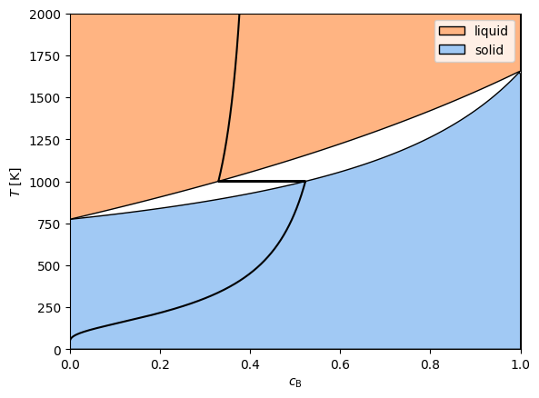
Set up some simple toy phase models that yields this phase diagram.

solid_a = LinePhase('A', fixed_concentration=0, line_energy=-2.0, line_entropy=1.0*kB)
solid_b = LinePhase('B', fixed_concentration=1, line_energy=-3.0, line_entropy=1.5*kB)

solid = IdealSolution('solid', solid_a, solid_b)

liquid_a = LinePhase('A(l)', fixed_concentration=0, line_energy=-1.9, line_entropy=2.5*kB)
liquid_b = LinePhase('B(l)', fixed_concentration=1, line_energy=-2.9, line_entropy=2.2*kB)

liquid = IdealSolution('liquid', liquid_a, liquid_b)

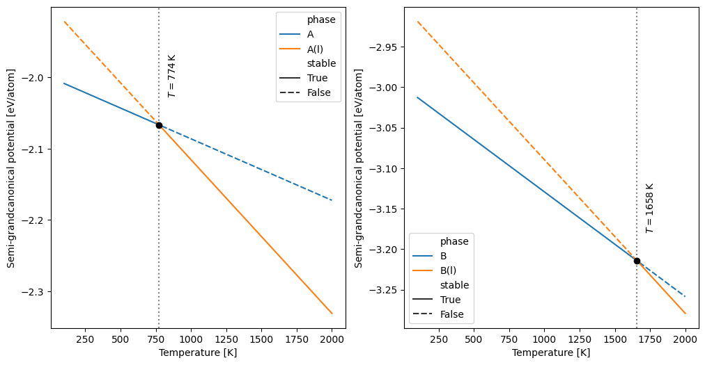
Examples for congruent melting

For the terminals and at fixed concentration, the chemical potential difference does not matter, so we can set it to zero. In this case the semigrand potential is equal to the free energy.

plt.figure(figsize=(12,6))
plt.subplot(121)
df = calc_phase_diagram([solid_a, liquid_a], Ts=np.linspace(100, 2000, 100), mu=0.0, keep_unstable=True)
plot_1d_T_phase_diagram(df, ax=plt.gca(), show=False)

plt.subplot(122)
df = calc_phase_diagram([solid_b, liquid_b], Ts=np.linspace(100, 2000, 100), mu=0.0, keep_unstable=True)
plot_1d_T_phase_diagram(df, ax=plt.gca(), show=False)

<Axes: xlabel='Temperature [K]', ylabel='Semi-grandcanonical potential [eV/atom]'>

Non-Congruent Melting

However, the general formulation in the semigrand ensemble allows us to also investigate non-congruent melting transitions using the exact same code and formalism.

To do this, let’s first find out, what’s the chemical potential difference where liquid and solid are in equilibrium at, say, 1000K.

T_twophase = 1000

df = calc_phase_diagram([solid, liquid], Ts=T_twophase, mu=1000, keep_unstable=True)

plot_1d_mu_phase_diagram(df)

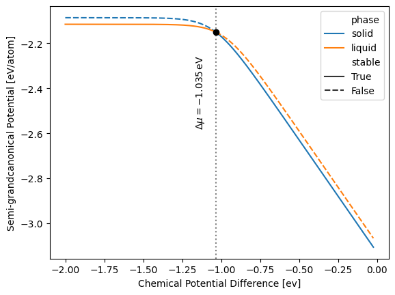
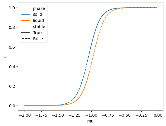
From the results, we can already get the concentrations on the liquidus and solidus, either by plot isotherms or numerically from the dataframe.

df.query('border')

	T	phase	phi	mu	c	stable	border	refined	f	f_excess
2000	1000	liquid	-2.149932	-1.035211	0.329906	True	True	mu	-2.491454	-0.041544
2001	1000	solid	-2.149932	-1.035211	0.522831	True	True	mu	-2.691173	-0.045672

mu_equilibrium_1000k = df.query('border').mu.iloc[0] # ~ -1.035 eV

mu_equilibrium_1000k

np.float64(-1.0352114196607491)

sns.lineplot(
    data=df,
    x='mu', y='c',
    hue='phase',
    style='stable', style_order=[True, False],
)
plt.axvline(mu_equilibrium_1000k, ls='dotted', c='k')

<matplotlib.lines.Line2D at 0x7f5e2bb7ea10>

Using the f and f_excess columns, we can also plot the more familiar common tangent construction.

sns.lineplot(
    data=df,
    x='c', y='f',
    hue='phase',
    style='stable', style_order=[True, False]
)
sns.lineplot(
    data=df.query('border'),
    x='c', y='f',
    ls='dotted', c='k'
)
sns.scatterplot(
    data=df.query('border'),
    x='c', y='f',
    c='k',
    zorder=2
)

<Axes: xlabel='c', ylabel='f'>

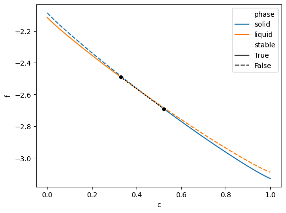
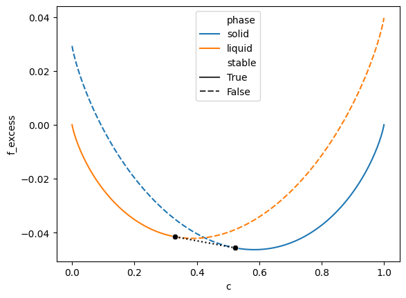
Difficult to see in \(f\) due to linear shift, let’s use \(f_\mathrm{excess}\) to see it more clearly.

sns.lineplot(
    data=df,
    x='c', y='f_excess',
    hue='phase',
    style='stable', style_order=[True, False]
)
sns.lineplot(
    data=df.query('border'),
    x='c', y='f_excess',
    ls='dotted', c='k'
)
sns.scatterplot(
    data=df.query('border'),
    x='c', y='f_excess',
    c='k',
    zorder=2
)

<Axes: xlabel='c', ylabel='f_excess'>

df = calc_phase_diagram([solid, liquid], Ts=np.linspace(0, 2000, 1000), mu=mu_equilibrium_1000k, keep_unstable=True, refine=True)

plot_1d_T_phase_diagram(df)

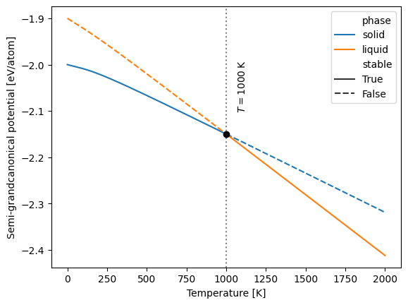
<Axes: xlabel='Temperature [K]', ylabel='Semi-grandcanonical potential [eV/atom]'>

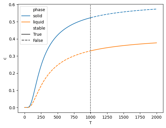
sns.lineplot(
    data=df,
    x='T', y='c',
    hue='phase',
    style='stable', style_order=[True, False],
)
plt.axvline(T_twophase, ls='dotted', c='k')

<matplotlib.lines.Line2D at 0x7f5e2a019a90>

Appendix: Inline Plots

Code that generates the pasted pictures above.

bdf = calc_phase_diagram([solid, liquid], Ts=np.linspace(0, 2000, 100), mu=200, keep_unstable=True)

Fig1

plt.figure(figsize=(12,6))
plt.subplot(121)
plot_phase_diagram(bdf, element='B', poly_method='fasttsp')
plt.subplot(122)
plot_mu_phase_diagram(bdf, element='B', poly_method='fasttsp')

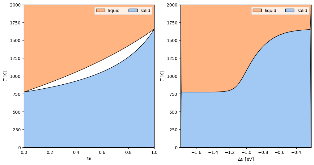
Fig3

T_twophase = 1000

df1000 = calc_phase_diagram([solid, liquid], Ts=1000, mu=1000, keep_unstable=True)
mu_equilibrium_1000k = df.query('border').mu.iloc[0]

plot_phase_diagram(bdf, element='B', poly_method='fasttsp')
plt.axhline(1000, ls='-', c='k')
sns.scatterplot(
    data=df1000.query('border'),
    x='c', y='T',
    marker='o', c='k'
)

<Axes: xlabel='$c_\\mathrm{B}$', ylabel='$T$ [K]'>

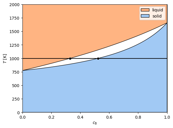
Fig2

dfisomu = calc_phase_diagram([solid, liquid], Ts=np.linspace(0, 2000, 1000), mu=mu_equilibrium_1000k, keep_unstable=True, refine=True)

plot_phase_diagram(bdf, element='B', poly_method='fasttsp')
sns.lineplot(
    data=dfisomu.query('stable'),
    x='c', y='T',
    orient='y', 
    # sort=False,
    estimator=None,
    c='k'
)

<Axes: xlabel='$c_\\mathrm{B}$', ylabel='$T$ [K]'>