Basics

Prelude

import landau.phases as ldp
import landau.interpolate as ldi
import landau.calculate as ldc
import landau.plot as lpl

import numpy as np
import matplotlib.pyplot as plt
import pandas as pd
import seaborn as sns

Temperature Transitions

Set up basic phases

ldp.LinePhase?

Init signature:
ldp.LinePhase(
    name: str,
    fixed_concentration: float,
    line_energy: float,
    line_entropy: float = 0,
) -> None
Docstring:      Simple phase with a fixed concentration and temperature independent entropy.
File:           ~/science/phd/dev/landau/landau/phases.py
Type:           ABCMeta
Subclasses:     

fcca = ldp.LinePhase("fccA", fixed_concentration=0, line_energy=-3, line_entropy=1*ldp.kB)
hcpa = ldp.LinePhase("hcp", fixed_concentration=0, line_energy=-2.975, line_entropy=1.8*ldp.kB)
lqda = ldp.LinePhase("liquidA", fixed_concentration=0, line_energy=-2.75, line_entropy=5*ldp.kB)

Landau does not know about units, but energies should be “per atom” or at least consistent among phases.

Just Plot Around

semigrand_potential is the main method. For dmu=0 it is the same as the free energy, otherwise

\[ \phi(\Delta\mu, T) = \min_c f(c, T) - c \Delta\mu \]

fcca.semigrand_potential?

Signature: fcca.semigrand_potential(T, dmu)
Docstring: Calculate the semigrand potential of the phase.
File:      ~/science/phd/dev/landau/landau/phases.py
Type:      method

Ts = np.linspace(0, 1000)

plt.plot(Ts, fcca.semigrand_potential(Ts, 0))
plt.plot(Ts, hcpa.semigrand_potential(Ts, 0))
plt.plot(Ts, lqda.semigrand_potential(Ts, 0))
plt.xlabel("$T$ [K]")
plt.ylabel(r"$f$/$\phi$ [eV/atom]")

Text(0, 0.5, '$f$/$\\phi$ [eV/atom]')

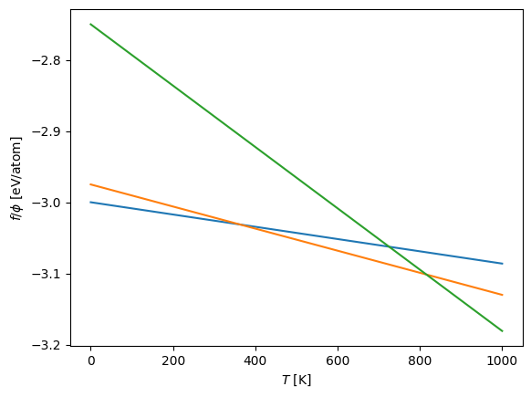
Crossing points are phase transitions. How to find them?

Ts = np.linspace(0, 1000, 10)

Simple call to just find stable phases at sample points.

df = ldc.calc_phase_diagram([fcca, hcpa, lqda], Ts, mu=0.0, refine=False)

Columns:

• phi semigrand potential

• mu chemical potential difference between both species

• stable True if a stable phase point

• f free energy corresponding to phi

• f_excess excess of the free energy wrt the stable phases

df

	T	phase	phi	mu	c	stable	f	f_excess
0	0.000000	fccA	-3.000000	0.0	0	True	-3.000000	0.0
1	111.111111	fccA	-3.009575	0.0	0	True	-3.009575	0.0
2	222.222222	fccA	-3.019150	0.0	0	True	-3.019150	0.0
3	333.333333	fccA	-3.028724	0.0	0	True	-3.028724	0.0
14	444.444444	hcp	-3.043939	0.0	0	True	-3.043939	0.0
15	555.555556	hcp	-3.061173	0.0	0	True	-3.061173	0.0
16	666.666667	hcp	-3.078408	0.0	0	True	-3.078408	0.0
17	777.777778	hcp	-3.095643	0.0	0	True	-3.095643	0.0
28	888.888889	liquidA	-3.132993	0.0	0	True	-3.132993	0.0
29	1000.000000	liquidA	-3.180867	0.0	0	True	-3.180867	0.0

Additionally refine the phase boundaries. Adds additional columns border and refined. border is True if the point is a phase transition. refined is a string telling how the point was added.

df = ldc.calc_phase_diagram([fcca, hcpa, lqda], Ts, mu=0.0, refine=True)

df

	T	phase	phi	mu	c	stable	border	refined	f	f_excess
0	0.000000	fccA	-3.000000	0.0	0	True	False	no	-3.000000	0.000000e+00
1	111.111111	fccA	-3.009575	0.0	0	True	False	no	-3.009575	0.000000e+00
2	222.222222	fccA	-3.019150	0.0	0	True	False	no	-3.019150	0.000000e+00
3	333.333333	fccA	-3.028724	0.0	0	True	False	no	-3.028724	0.000000e+00
4	444.444444	hcp	-3.043939	0.0	0	True	False	no	-3.043939	0.000000e+00
5	555.555556	hcp	-3.061173	0.0	0	True	False	no	-3.061173	0.000000e+00
6	666.666667	hcp	-3.078408	0.0	0	True	False	no	-3.078408	0.000000e+00
7	777.777778	hcp	-3.095643	0.0	0	True	False	no	-3.095643	0.000000e+00
8	888.888889	liquidA	-3.132993	0.0	0	True	False	no	-3.132993	0.000000e+00
9	1000.000000	liquidA	-3.180867	0.0	0	True	False	no	-3.180867	0.000000e+00
30	362.641191	fccA	-3.031250	0.0	0	True	True	T	-3.031250	0.000000e+00
31	362.641191	hcp	-3.031250	0.0	0	True	True	T	-3.031250	0.000000e+00
32	815.942680	hcp	-3.101562	0.0	0	True	True	T	-3.101562	4.440892e-16
33	815.942680	liquidA	-3.101563	0.0	0	True	True	T	-3.101563	0.000000e+00

keep_unstable can be passed to also retain samples of the unstable phases.

df = ldc.calc_phase_diagram([fcca, hcpa, lqda], Ts, mu=0.0, refine=True, keep_unstable=True)

df

	T	phase	phi	mu	c	stable	border	refined	f	f_excess
0	0.000000	fccA	-3.000000	0.0	0	True	False	no	-3.000000	0.000000e+00
1	111.111111	fccA	-3.009575	0.0	0	True	False	no	-3.009575	0.000000e+00
2	222.222222	fccA	-3.019150	0.0	0	True	False	no	-3.019150	0.000000e+00
3	333.333333	fccA	-3.028724	0.0	0	True	False	no	-3.028724	0.000000e+00
4	444.444444	hcp	-3.043939	0.0	0	True	False	no	-3.043939	0.000000e+00
5	555.555556	hcp	-3.061173	0.0	0	True	False	no	-3.061173	0.000000e+00
6	666.666667	hcp	-3.078408	0.0	0	True	False	no	-3.078408	0.000000e+00
7	777.777778	hcp	-3.095643	0.0	0	True	False	no	-3.095643	0.000000e+00
8	888.888889	liquidA	-3.132993	0.0	0	True	False	no	-3.132993	0.000000e+00
9	1000.000000	liquidA	-3.180867	0.0	0	True	False	no	-3.180867	0.000000e+00
10	444.444444	fccA	-3.038299	0.0	0	False	False	NaN	-3.038299	5.639407e-03
11	555.555556	fccA	-3.047874	0.0	0	False	False	NaN	-3.047874	1.329926e-02
12	666.666667	fccA	-3.057449	0.0	0	False	False	NaN	-3.057449	2.095911e-02
13	777.777778	fccA	-3.067024	0.0	0	False	False	NaN	-3.067024	2.861896e-02
14	888.888889	fccA	-3.076599	0.0	0	False	False	NaN	-3.076599	5.639407e-02
15	1000.000000	fccA	-3.086173	0.0	0	False	False	NaN	-3.086173	9.469333e-02
16	0.000000	hcp	-2.975000	0.0	0	False	False	NaN	-2.975000	2.500000e-02
17	111.111111	hcp	-2.992235	0.0	0	False	False	NaN	-2.992235	1.734015e-02
18	222.222222	hcp	-3.009469	0.0	0	False	False	NaN	-3.009469	9.680296e-03
19	333.333333	hcp	-3.026704	0.0	0	False	False	NaN	-3.026704	2.020445e-03
20	888.888889	hcp	-3.112877	0.0	0	False	False	NaN	-3.112877	2.011526e-02
21	1000.000000	hcp	-3.130112	0.0	0	False	False	NaN	-3.130112	5.075466e-02
22	0.000000	liquidA	-2.750000	0.0	0	False	False	NaN	-2.750000	2.500000e-01
23	111.111111	liquidA	-2.797874	0.0	0	False	False	NaN	-2.797874	2.117007e-01
24	222.222222	liquidA	-2.845748	0.0	0	False	False	NaN	-2.845748	1.734015e-01
25	333.333333	liquidA	-2.893622	0.0	0	False	False	NaN	-2.893622	1.351022e-01
26	444.444444	liquidA	-2.941496	0.0	0	False	False	NaN	-2.941496	1.024424e-01
27	555.555556	liquidA	-2.989370	0.0	0	False	False	NaN	-2.989370	7.180296e-02
28	666.666667	liquidA	-3.037244	0.0	0	False	False	NaN	-3.037244	4.116356e-02
29	777.777778	liquidA	-3.085119	0.0	0	False	False	NaN	-3.085119	1.052415e-02
30	362.641191	fccA	-3.031250	0.0	0	True	True	T	-3.031250	0.000000e+00
31	362.641191	hcp	-3.031250	0.0	0	True	True	T	-3.031250	0.000000e+00
32	815.942680	hcp	-3.101562	0.0	0	True	True	T	-3.101562	4.440892e-16
33	815.942680	liquidA	-3.101563	0.0	0	True	True	T	-3.101563	0.000000e+00

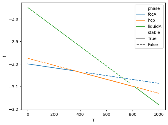
A simple plot with seaborn.

sns.lineplot(
    data=df,
    x='T', y='f',
    hue='phase',
    style='stable', style_order=[True, False],
)

<Axes: xlabel='T', ylabel='f'>

Or using landau

lpl.plot_1d_T_phase_diagram(df)

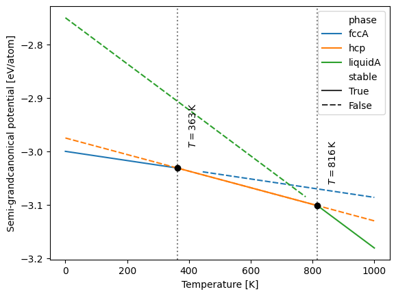
<Axes: xlabel='Temperature [K]', ylabel='Semi-grandcanonical potential [eV/atom]'>

Including Concentration

landau implicitly assumes there is only two species and that all phase objects agree on which is the ‘first’ and which is the ‘second’.

Phase objects with variable concentration are most easily assembled from objects of fixed concentration, because this is how e.g. calphy presents them.

fccb = ldp.LinePhase("fccB", fixed_concentration=1, line_energy=-2, line_entropy=1.1*ldp.kB)

hcpb = ldp.LinePhase("hcpB", fixed_concentration=1, line_energy=-1.95, line_entropy=1.1*ldp.kB)

fcc = ldp.IdealSolution('fcc', fcca, fccb)

hcp = ldp.IdealSolution('hcp', hcpa, hcpb)

All phases present the same interface to calculate the semi-grandcanonical potential.

fcc.semigrand_potential?

Signature: fcc.semigrand_potential(T, dmu)
Docstring: Calculate the semigrand potential of the phase.
File:      ~/science/phd/dev/landau/landau/phases.py
Type:      method

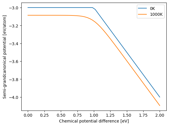
mus = np.linspace(0, 2)

plt.plot(mus, fcc.semigrand_potential(   0, mus), label='0K')
plt.plot(mus, fcc.semigrand_potential(1000, mus), label='1000K')
plt.xlabel("Chemical potential difference [eV]")
plt.ylabel("Semi-grandcanonical potential [eV/atom]")
plt.legend()

<matplotlib.legend.Legend at 0x7fd7c26c1b90>

Chemical potential range can also be guessed.

ldc.guess_mu_range([fcc], T=1000, samples=100)

(array([0.20348167, 0.59702767, 0.65649822, 0.69224108, 0.71784655,
        0.73785687, 0.75505521, 0.76873383, 0.7816471 , 0.79224485,
        0.8028426 , 0.81167202, 0.82000879, 0.82834556, 0.83561447,
        0.84230052, 0.84898658, 0.85567263, 0.86147831, 0.86697089,
        0.87246348, 0.87795607, 0.88344865, 0.88811217, 0.89275789,
        0.89740361, 0.90204934, 0.90669506, 0.91113655, 0.9152035 ,
        0.91927046, 0.92333741, 0.92740436, 0.93147132, 0.93553827,
        0.93926782, 0.94297044, 0.94667306, 0.95037569, 0.95407831,
        0.95778093, 0.96148355, 0.96502695, 0.9685459 , 0.97206486,
        0.97558381, 0.97910276, 0.98262172, 0.98614067, 0.98965083,
        0.99314975, 0.99664867, 1.0001476 , 1.00364652, 1.00714544,
        1.01064436, 1.01414329, 1.01777959, 1.02142026, 1.02506093,
        1.0287016 , 1.03234227, 1.03598294, 1.03962362, 1.04351443,
        1.04747176, 1.0514291 , 1.05538644, 1.05934378, 1.06330112,
        1.06735489, 1.07183317, 1.07631146, 1.08078974, 1.08526802,
        1.0897463 , 1.09449426, 1.09974606, 1.10499786, 1.11024966,
        1.11550146, 1.12116141, 1.127511  , 1.1338606 , 1.14021019,
        1.14694898, 1.15482242, 1.16269587, 1.17056931, 1.18039948,
        1.1903641 , 1.20122061, 1.21403758, 1.22791481, 1.24460976,
        1.26503001, 1.29068089, 1.32576234, 1.38630569, 1.78603808]),
 np.float64(0.00010701744583500724),
 np.float64(0.9998999870320691))

mus, *_ = ldc.guess_mu_range([fcc], T=1000, samples=100)

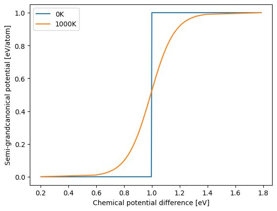
Isothermals are available via the concentration method.

fcc.concentration?

Signature: fcc.concentration(T, dmu)
Docstring: Concentration of the phase at the given state.
File:      ~/science/phd/dev/landau/landau/phases.py
Type:      method

plt.plot(mus, fcc.concentration(   0, mus), label='0K')
plt.plot(mus, fcc.concentration(1000, mus), label='1000K')
plt.xlabel("Chemical potential difference [eV]")
plt.ylabel("Semi-grandcanonical potential [eV/atom]")
plt.legend()

<matplotlib.legend.Legend at 0x7fd7c25525d0>

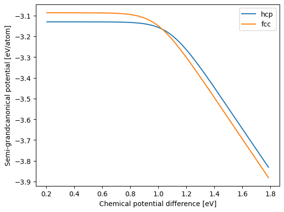
Again, phase transitions are determined by the intersection points.

plt.plot(mus, hcp.semigrand_potential(1000, mus), label='hcp')
plt.plot(mus, fcc.semigrand_potential(1000, mus), label='fcc')
plt.xlabel("Chemical potential difference [eV]")
plt.ylabel("Semi-grandcanonical potential [eV/atom]")
plt.legend()

<matplotlib.legend.Legend at 0x7fd7ba12be90>

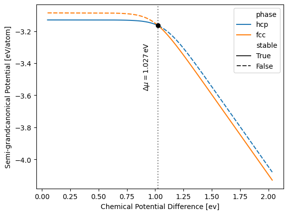
df = ldc.calc_phase_diagram([hcp, fcc], Ts=1000, mu=100, keep_unstable=True)

lpl.plot_1d_mu_phase_diagram(df)

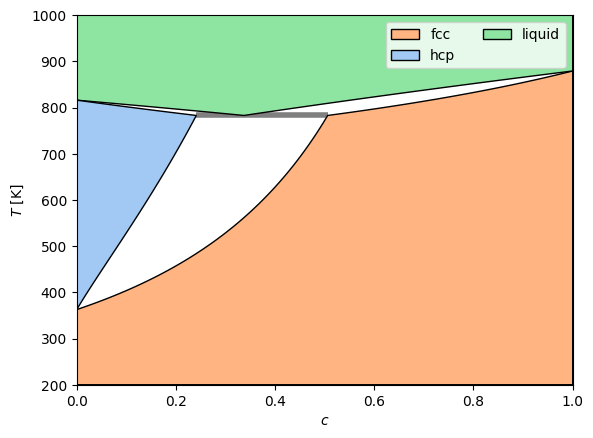
Adding a liquid phase as well and finally plotting the full diagram.

lqdb = ldp.LinePhase("liquidB", fixed_concentration=1, line_energy=-1.75, line_entropy=4.4*ldp.kB)
lqd = ldp.IdealSolution('liquid', lqda, lqdb)

%%time
Ts = np.linspace(200, 1000)
df = ldc.calc_phase_diagram([hcp, fcc, lqd], Ts, mu=100)

CPU times: user 1.32 s, sys: 5.93 ms, total: 1.33 s
Wall time: 1.33 s

df

	T	phase	phi	mu	c	stable	border	refined	f	f_excess
0	363.265306	hcp	-3.031347	0.053318	1.641792e-14	True	False	no	-3.031347	-1.643130e-14
1	363.265306	hcp	-3.031347	0.645306	2.680972e-06	True	False	no	-3.031345	-1.026572e-06
2	363.265306	hcp	-3.031347	0.706245	1.878120e-05	True	False	no	-3.031334	-6.047016e-06
3	363.265306	hcp	-3.031349	0.742431	5.966762e-05	True	False	no	-3.031304	-1.705217e-05
4	363.265306	hcp	-3.031351	0.768429	1.368946e-04	True	False	no	-3.031246	-3.556378e-05
...	...	...	...	...	...	...	...	...	...	...
15708	798.894454	liquid	-3.107717	0.936009	1.780641e-01	True	True	delaunay	-2.941047	4.468980e-02
15709	798.894454	hcp	-3.107717	0.936009	1.199755e-01	True	True	delaunay	-2.995419	-6.523235e-03
15710	782.832625	fcc	-3.115044	0.994895	5.060824e-01	True	True	delaunay-triple	-2.611545	1.301759e-01
15711	782.832625	liquid	-3.115044	0.994895	3.372285e-01	True	True	delaunay-triple	-2.779537	6.686710e-03
15712	782.832625	hcp	-3.115044	0.994895	2.411723e-01	True	True	delaunay-triple	-2.875103	-6.356284e-02

5713 rows × 10 columns

lpl.plot_phase_diagram(df, tielines=True, poly_method='fasttsp')

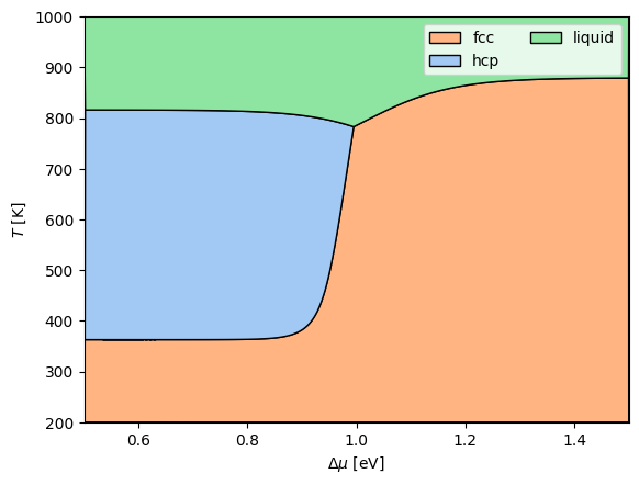
Can also plot in mu/T space.

%%time
Ts = np.linspace(200, 1000, 200)
mus = np.linspace(0.5, 1.5, 200)
df = ldc.calc_phase_diagram([hcp, fcc, lqd], Ts, mu=mus)

CPU times: user 3.8 s, sys: 29 ms, total: 3.83 s
Wall time: 3.85 s

%%time
lpl.plot_mu_phase_diagram(df)

CPU times: user 15.1 s, sys: 26.6 ms, total: 15.1 s
Wall time: 12.1 s